Audio Generation using WGANs

I've always wanted to be able to find a method to generate audio. I looked at examples on the internet, but either they sounded like TV Static, or only had the ability to produce a singular note, such as in the case of GanSynth or WaveGAN. In this blog post I'll be going over how to generate 5s audio clips from a GAN, but not just any GAN, a Wasserstein GAN.

Getting the Audio Data

Firstly, we need to fetch the audio data. I used a LoFi music compilation, but feel free to use any type of music compilation on or off youtube. After that, I used yt-dlp, an open-source project to get the mp3 from the youtube URL. Here is the following command:

yt-dlp -x --audio-format mp3 <video_url>

Now you can go ahead and use any tool to split this mp3 file into (preferably) 5 second segments. Next, we need to be able to take these audio segments and create images out of them. For this, we will use a python library called Librosa, which has very useful audio manipulation utilities. Below is a method to load in an audio file in array format given the file path.

def load_audio(self, audio_file=None, raw_audio=None):
        """
        x_res: width of resulting spectrogram image
        hop_length: number of samples between successive frames
        """
        if audio_file is not None:
            #using librosa and loading audio, given sample size
            self.audio, _ = librosa.load(audio_file, mono=True, sr=self.sr)
        else:
            self.audio = raw_audio

        if len(self.audio) < self.x_res * self.hop_length:
            #add padding if the length of audio doesn't match up with the expected length
            self.audio = np.concatenate([self.audio, np.zeros((self.x_res * self.hop_length - len(self.audio),))])

This is a method from a class that allows us to perform whatever audio manipulation needed. First, we use librosa.load() to load in our audio file, with a set sampling rate of 22050. After that, we need to pad our audio array so that it's at a fixed length. We want the length of the audio to be our spectrogram width times the hop length, so that when we create our spectrogram, it adheres to the horizontal resolution of the image. So we pad it with additional 0s to cover up that space as done with np.concatenate().

Next, we want to be able to convert from padded audio array to an image or a tensor. For that we will be utilizing a Mel spectrogram. Here's what the method looks like.

def audio_slice_to_image(self, slice, ref=np.max):
        #get mel spectrogram of audio
        S = librosa.feature.melspectrogram(
            y=self.get_audio_slice(slice), sr=self.sr, n_fft=self.n_fft, hop_length=self.hop_length, n_mels=self.n_mels
        )
        #convert spectrogram to decibels and specify the top decibel
        log_S = librosa.power_to_db(S, ref=ref, top_db=self.top_db)
        #compress and clip the db spectrogram into suitable range for image
        bytedata = (((log_S + self.top_db) * 255 / self.top_db).clip(0, 255) + 0.5).astype(np.uint8)
        #convert array into image and return
        image = Image.fromarray(bytedata)
        return image

We first use librosa.feature.melspectrogram() to actually get the mel spectrogram. In our next line, we use librosa to convert our mel spectrogram into a decibel spectrogram, which is a visual representation of the decibel values in our mel spectrogram. We specify two values ref and top_db. The first value, ref is the baseline decibel value that we want when converting our mel spectrogram, and here it's equal to the maximum value of the Mel spectrogram. Then we specify our top decibel value in the top_db argument.

Now we have essentially restricted our audio representation into a range. But we need that range to be between [0, 255] so that we can convert it into an image. We use some math, along with clipping values to achieve this. To convert the array into an image, I used the Python Image Library (PIL).

Now we want to be able to convert from image back to audio. We can just reverse all the steps that we used in the method above.

def image_to_audio(self, image):
        bytedata = np.frombuffer(image.tobytes(), dtype="uint8").reshape((image.height, image.width))
        log_S = bytedata.astype("float") * self.top_db / 255 - self.top_db
        S = librosa.db_to_power(log_S)
        audio = librosa.feature.inverse.mel_to_audio(
            S, sr=self.sr, n_fft=self.n_fft, hop_length=self.hop_length, n_iter=self.n_iter
        )
        return audio

As you can see here, we first convert to image back into a tensor. Then we reverse our steps to get back the Mel spectrogram. We can utilize the librosa.feature.inverse.mel_to_audio() method to convert our spectrogram back into our audio array.

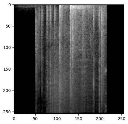
Now we can use these methods to convert all the files in our directory into images. In my case, I'm converting them to tensor data, which only takes a few modifications from the code above. Then we save all this tensor data into a binary file. Also make sure to normalize the tensor data between -1 and 1, since that's what the GAN architecture will need. Here's what a sample image looks like for my dataset:

GAN Architecture

Now we will create our GAN architecture. The high level overview is we have a generator that accepts a noise vector, reshapes it into some 3D tensor, and then continuously upsample it to our image size of 256x256. For the discriminator we do the opposite, taking in the image then downsampling it enough times, then flattening it and running it through a MLP. For the generator, I will be using an upsample block, which includes batch normalization. Likewise for the discriminator I will be using a downsample block. If you want to see the code for them, along with the full code, check out the repo at the bottom of the article. Anyways, here's the generator architecture.

def get_generator_model():
    #define input to be the noise dim
    noise = layers.Input(shape=(noise_dim,))
    #reshape to 8x8x1024 to pass into upsample blocks
    x = layers.Dense(8 * 8 * 1024, use_bias=False)(noise)
    x = layers.BatchNormalization()(x)
    x = layers.LeakyReLU(0.2)(x)
    x = layers.Reshape((8, 8, 1024))(x)
    #8x8x1024 --> 16x16x512
    x = upsample_block(x, 512, layers.LeakyReLU(0.2), strides=(1, 1), use_bias=False, use_bn=True, padding="same", use_dropout=False)
    #16x16x512 --> 32x32x256
    x = upsample_block(x, 256, layers.LeakyReLU(0.2), strides=(1, 1), use_bias=False, use_bn=True, padding="same", use_dropout=False)
    #32x32x256 --> 64x64x128
    x = upsample_block(x, 128, layers.LeakyReLU(0.2), strides=(1, 1), use_bias=False, use_bn=True, padding="same", use_dropout=False)
    #64x64x126 --> 128x128x64
    x = upsample_block(x, 64, layers.LeakyReLU(0.2), strides=(1, 1), use_bias=False, use_bn=True, padding="same", use_dropout=False)
    #128x128x64 --> 256x256x1
    x = upsample_block(x, 1, layers.Activation("tanh"), strides=(1, 1), use_bias=False, use_bn=True)
    #define model
    g_model = keras.models.Model(noise, x, name="generator")
    return g_model

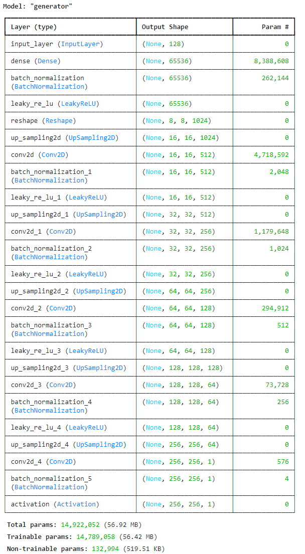
We can see here that first, our generator accepts an input vector, then it uses a dense layer to upsample it to a 8x8x1024 tensor. Then we continuously apply our upsample block, until we have achieved our image size, and we use the tanh activation function, to restrict it between [-1, 1]. Here is an image encapsulating the architecture of our model, along with some additional information.

Now let's take a look at our discriminator architecture:

def get_discriminator_model():
    img_input = layers.Input(shape=IMG_SHAPE)
    #256x256x1 --> 128x128x64
    x = conv_block(img_input, 64, kernel_size=(5, 5), strides=(2, 2), use_bn=False, use_bias=True, activation=layers.LeakyReLU(0.2), use_dropout=False, drop_value=0.3)
    #128x128x64 --> 64x64x128
    x = conv_block(x, 128, kernel_size=(5, 5), strides=(2, 2), use_bn=False, use_bias=True, activation=layers.LeakyReLU(0.2), use_dropout=True, drop_value=0.3)
    #64x64x128 --> 32x32x256
    x = conv_block(x, 256, kernel_size=(5, 5), strides=(2, 2), use_bn=False, use_bias=True, activation=layers.LeakyReLU(0.2), use_dropout=True, drop_value=0.3)
    #32x32x256 --> 16x16x512
    x = conv_block(x, 512, kernel_size=(5, 5), strides=(2, 2), use_bn=False, use_bias=True, activation=layers.LeakyReLU(0.2), use_dropout=False, drop_value=0.3)
    #flatten and output score
    x = layers.Flatten()(x)
    x = layers.Dropout(0.2)(x)
    x = layers.Dense(1)(x)

    d_model = keras.models.Model(img_input, x, name="discriminator")
    return d_model

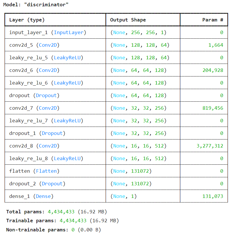
Here we first accept our image, and then continuously downsample it. Then we flatten the resulting tensor and pass it through one MLP layer, getting a score for the image. For the fellow ML Engineers out there you might notice that the final layer has no sigmoid activation function. This is because instead of classifying real and fake images, the discriminator or critic I should say, assigns a score to that image, which can have any range. This is what the architecture is like:

WGAN Implementation

Before implementing the WGAN, we need to talk about some differences betwee WGANs and GANs. The type of WGAN I'm using involves a Gradient Penalty, so it's a WGAN-GP type. WGAN focuses on minimizing the Wasserstein distance (also known as Earth Mover's distance) between the distribution of generated data and the real data distribution. Meanwhile, GANs aim to train a generator network to produce data that is indistinguishable from real data, while a discriminator network tries to differentiate between real and fake data. They also have different loss functions. WGANs are generally more stable during training and are less prone to mode collapse, which is where the generator just produces the same output over and over again.

Now we need to actually implement our losses and backpropagation for the WGAN. Following is how to calculate the gradient penalty. Let's go through it along with supporting equations.

def gradient_penalty(self, batch_size, real_images, fake_images):
        alpha = tf.random.normal([batch_size, 1, 1, 1], 0.0, 1.0) #used to interpolate between real and fake images
        diff = fake_images - real_images #difference in real and fake images
        interpolated = real_images + alpha * diff #creates interpolated images

        #record operations to compute gradients
        with tf.GradientTape() as gp_tape:
            gp_tape.watch(interpolated)
            #make discriminator prediction on interpolated images
            pred = self.discriminator(interpolated, training=True)

        grads = gp_tape.gradient(pred, [interpolated])[0] #gradient of discriminator's predictions with respect to interpolated images
        norm = tf.sqrt(tf.reduce_sum(tf.square(grads), axis=[1, 2, 3])) #calculates euclidean norm of gradients
        gp = tf.reduce_mean((norm - 1.0) ** 2) #calculates gradient penalty
        return gp

Firstly, let's establish a mean function $m(x)=\frac{\sum{x}}{N}$ that just calculates the average of a given tensor across all axes. We also calculate our fake images with $G(z_{i}) = x_{i}$, where G is the forward pass of the generator. The first line generates a tensor sampled from the normal distribution and can be represented with $\alpha \sim \mathcal{N}(0,1)$, since we are taking it from the normal distribution. After that, we calculate the interpolated images, which is what the discriminator will predict off of. The equation for it is:

This equation just representes the code, in which we add the real images to the difference between the fake and real images times our randomly generated tensor. Next we use this to make a prediction using our discriminator. It looks like $P_{i}=D(I_{i})$, where D is a function representing the discriminator's forward pass. Next we calculate the gradient, which is $g = \frac{\partial{P}}{\partial{I}}$. This is what we are doing in the code, using the measurements from the gp_tape to calculate our gradient.

Then we find the euclidean norm of the gradient, and using that we calculate the gradient penalty using this complicated-looking equation: $GP = m({(\sqrt{\sum{g^2}}-1)^2})$. In reality this just applies many simple operations together. Now that we have the gradient penalty, let's look at the loss functions for the discriminator and generator.

The loss function for the generator is $L_{G}(\hat{x}) = -m({D(\hat{x})})$. Let's think about why it works. We want the discriminator prediction to be as positive as possible, so to lower the loss for the generator, since the discriminator has been fooled. For the discriminator its loss is $C_{D}(x, \hat{x}) = m({D(\hat{x})}) - m({D(x)})$. This is also very self explanatory, as it wants to assign negative scores to fake images, and positive ones to real images. The following is the code for the functions, along with the optimizers.

generator_optimizer = keras.optimizers.Adam(
	learning_rate=0.0002, beta_1=0.5, beta_2=0.9)

discriminator_optimizer = keras.optimizers.Adam(
    learning_rate=0.0002, beta_1=0.5, beta_2=0.9)

def discriminator_loss(real_img, fake_img):
    real_loss = tf.reduce_mean(real_img)
    fake_loss = tf.reduce_mean(fake_img)
    return fake_loss - real_loss

def generator_loss(fake_img):
    return -tf.reduce_mean(fake_img)

Now we can implement the entire call function for the WGAN Model Class:

def train_step(self, real_images):
        #deal with tuples
        if isinstance(real_images, tuple):
            real_images = real_images[0]
        #get batch size by looking at axis 0
        batch_size = tf.shape(real_images)[0]

        #train discriminator d_steps times
        for i in range(self.d_steps):
            random_latent_vectors = tf.random.normal(
                shape=(batch_size, self.latent_dim)
            ) #generate noise
            #tape for calculating gradients
            with tf.GradientTape() as tape:
                fake_images = self.generator(random_latent_vectors, training=True) #generate fake images
                #get discriminator predictions on fake images
                fake_logits = self.discriminator(fake_images, training=True)
                #get discriminator predictions on real images
                real_logits = self.discriminator(real_images, training=True)
                #calculate normal loss, just like a GAN
                d_cost = self.d_loss_fn(real_img=real_logits, fake_img=fake_logits)
                #find gradient penalty
                gp = self.gradient_penalty(batch_size, real_images, fake_images)
                #add back to loss
                d_loss = d_cost + gp * self.gp_weight
            #find gradient using loss and parameters
            d_gradient = tape.gradient(d_loss, self.discriminator.trainable_variables)
            #apply the gradients to model
            self.d_optimizer.apply_gradients(zip(d_gradient, self.discriminator.trainable_variables))
        #generate noise
        random_latent_vectors = tf.random.normal(shape=(batch_size, self.latent_dim))
        with tf.GradientTape() as tape:
            generated_images = self.generator(random_latent_vectors, training=True) #get generated images
            #get discriminator predictions on fake images
            gen_img_logits = self.discriminator(generated_images, training=True)
            #calculate generator loss using them
            g_loss = self.g_loss_fn(gen_img_logits)

        gen_gradient = tape.gradient(g_loss, self.generator.trainable_variables)

        self.g_optimizer.apply_gradients(zip(gen_gradient, self.generator.trainable_variables))
        return {"d_loss": d_loss, "g_loss": g_loss} #return losses

It's really long and complicated so let's break it down into steps:

1. Deal with tuples and get batch size
2. Train the discriminator d_steps times more than generator, that's why the for loop is there
3. Generate random noise from normal distribution
4. Generate fake images, and run them through the discriminator to get their scores
5. Run the real images through the discriminator and get the scores
6. Calculate the loss from the given functions above
7. Calculate the gradient penalty
8. Get the total discriminator loss using part of the loss and gradient penalty using this equation: $L_{D}(x, \hat{x}) = C_{D}(x, \hat{x}) + \lambda \times GP$. Here $\lambda$ is a constant called the GP weight, generally set to 0.10
9. Backpropagate the loss through the discriminator and get the gradients
10. Use the optimizer to apply the gradients to the discriminator
11. Repeat steps 3, 4, 6, 9, 10 for the generator

Training and Inference

The hard part is now done, we can just train the model now by fitting on the training data from the binary file. We first initialize the model, then we compile it. After that we just train the model. Then we save the weights for inference.

epochs = 30

wgan = WGAN(discriminator=d_model,
			generator=g_model,
            latent_dim=noise_dim,
            discriminator_extra_steps=3)

wgan.compile(d_optimizer=discriminator_optimizer,
			 g_optimizer=generator_optimizer,
             g_loss_fn=generator_loss,
             d_loss_fn=discriminator_loss,)
wgan.fit(train_images, batch_size=BATCH_SIZE, epochs=epochs, callbacks=[cbk])
wgan.save_weights('lofi_gen.weights.h5')

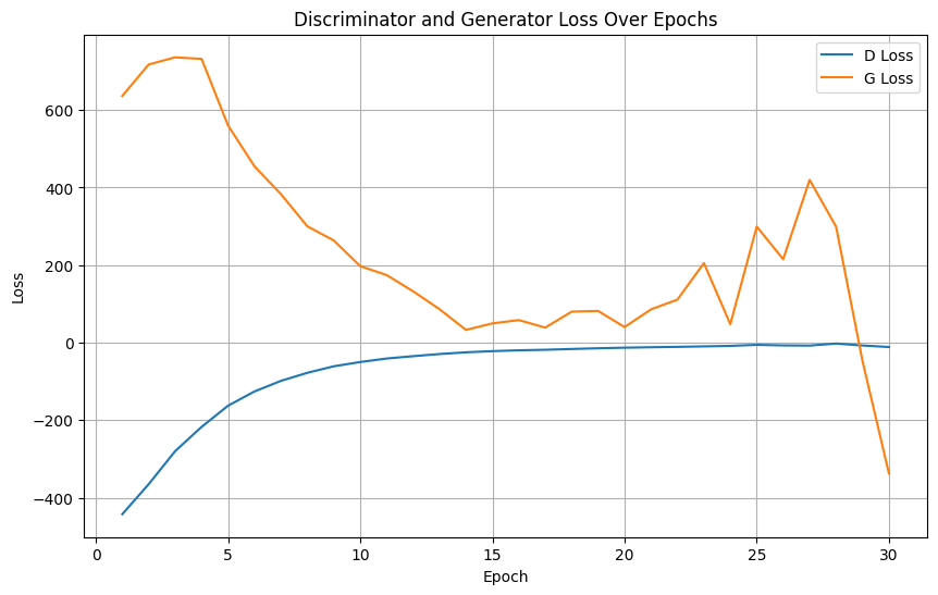
Here is a graph of the loss of the generator and discriminator:

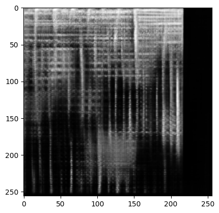
And here is a generated spectrogram from the model:

Now let's use Soundfile, PyDub and IPython to create a basic script to generate audio!

def generate():
    random_latent_vectors = tf.random.normal(shape=(1, noise_dim))
    generated_images = wgan.generator(random_latent_vectors, training=False)
    generated_images = (generated_images * 127.5) + 127.5
    #use mel to generate into audio
    aud = mel.vector_to_audio(np.array(generated_images[0], dtype=np.uint8))
    #save to file
    sf.write("gened_aud.wav", aud, 22050)
    #load back and amplify the audio
    audio = AudioSegment.from_wav("/kaggle/working/gened_aud.wav")
    amplified_audio = audio + 25
    #resave
    amplified_audio.export(f"gened_aud_ampl.wav", format="wav")
generate()
Audio("/kaggle/working/gened_aud_ampl.wav", autoplay=True) #play the audio from file

Here are the steps for this function:

• Generate random noise, and get the generated spectrogram from them using the WGAN's generator
• Use a vector_to_audio method similar to image_to_audio from before to convert the tensor into an audio array
• Use soundfile to write the array to a file
• Reopen the file, and increase the volume by 25 decibels
• Save the file then display it on the notebook output

Here are some sample sounds, and one of them below:

There are some times in the audio where it breaks apart and has issues, but in most spectrograms it's not a big issue and sounds decent, and in some of them, it sounds almost perfect!

Thanks for reading this! This is my first blogpost I've written so feedback would be encouraged. Also I didn't have the chance to talk about the entire code, so you can check it out on GitHub.